.h5 File Format

Measurements that use the recommended .h5 file saving strategy generate .h5 files that contain the data along with data structures that include all the metadata from the microscope app.

To view .h5 file data, we can:

• Use a graphical viewer like HDFView, or VSCode extensions like the one of h5web
• Use the FoundryDataBrowser from the ScopeFoundry project, or
• Make your own viewer.
• Use a Analyze with ipynb or see bellow.

Example

The data file created by the sine_wave_plot measurement has the following hierarchy:

|> app
    |- name = vfunc_gen_test_app
    |- ScopeFoundry_type = App
    |> settings
        |- save_dir = ~/fancy_microscope/data
        |- sample = Test Sample 42
        |> units
|> hardware
    |- ScopeFoundry_type = HardwareList
    |> virtual_function_gen
        |- name = virtual_function_gen
        |- ScopeFoundry_type = Hardware
        |> settings
            |- connected = True
            |- debug_mode = False
            |- amplitude = 1.0
            |- rand_data = 0.5191185618096453
            |- sine_data = 0.9099735972719286
            |- square_data = -1.0
            |> units
|> measurement
    |> sine_wave_plot
        |- name = sine_wave_plot
        |- ScopeFoundry_type = Measurement
        |D buffer: (120,) float64
        |> settings
            |- activation = False
            |- running = True
            |- progress = 50.0
            |- save_h5 = True
            |- sampling_period = 0.1
            |> units
                |- progress = %
                |- sampling_period = s

You will notice that this data file contains much more than just the sine wave data recorded during your measurement. It also contains all the settings of the hardware and measurement conditions at the time of the data acquisition.

We can access this data file in Python using the h5py package.

import h5py

dat = h5py.File('1486144636_sine_wave_plot.h5', 'r')

sample_name = dat['app/settings'].attrs['sample']
print(sample_name)
# Test Sample 42

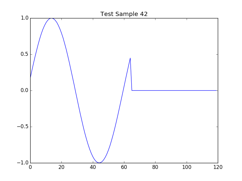
buffer_data = dat['measurement/sine_wave_plot/buffer']

import matplotlib.pyplot as plt
plt.title(sample_name)
plt.plot(buffer_data)
plt.savefig('sine_wave_data_plot_42.png')
plt.show()